로지스틱 회귀모형을 사용한 율의 표준화 방법: 국민건강보험공단 건강검진코호트 사용
Illustration of Calculating Standardized Rates Utilizing Logistic Regression Models: The National Health Insurance Service-National Health Screening Cohort (NHIS-HEALS)
Article information
Trans Abstract
Objectives
To illustrate an approach for standardizing rates utilizing logistic regression models that leads to the enhanced reliability of estimation with reduced calculation cost.
Methods
For illustrative purposes, data regarding metabolic syndrome patients in 2013 were extracted from the National Health Insurance Service-National Health Screening Cohort (NHIS-HEALS). The detailed step-by-step calculations of age-sex adjusted prevalence rates of metabolic syndrome were demonstrated by both direct and logistic regression standardization approaches whose results were then compared.
Results
Standardization of rates using logistic regression models facilitated relatively simple calculation that can be easily implemented by using widely employed analytical programs such as R, SPSS, and SAS. Treating age as a continuous variable, the logistic regression approach produced confidence intervals of age-sex adjusted prevalence rates that were much narrower as compared to confidence intervals obtained by the direct standardization.
Conclusions
Standardization of rates utilizing logistic regression models may be a competitive alternative to the direct standardization in terms of computational efficiency and estimation reliability.
서 론
보건·역학 관련 연구에서는 서로 다른 모집단에서 산출한 통계량을 비교하게 된다. 예를 들면, 어떤 한 지역의 유병률이 다른 지역보다 높은지 또는 어떤 지역의 특정 질병의 원인이 무엇인지를 밝히고자 할 때가 있다[1]. 대부분의 선행 연구를 통해 연령은 건강수준에 영향을 미치는 중요한 요인으로 알려져 있으므로[2,3], 지역별 차이를 연구할 때, 지역별 모집단의 상이한 연령 구조를 고려해야 한다[4]. 이와 같이 인구학적(demographic) 구조(성별, 사회·경제적 지위, 인종 등)의 지역 별 차이는 건강관련 지표를 산출하는 데 영향을 미친다. 인구학적 구조가 다른 지역 간 또는 기간별 유병률을 비교할 때, 연구의 주요 관심 대상이 아닌 교란변수(confounding variable)의 효과를 제거하고 지역 간 비교를 단순화시켜주는 지표로 표준화(standardization)를 사용한다. 표준화율(age-adjusted rate)은 1844년 사망률 자료를 분석하는 연구에서 처음으로 사용되었고[5], 이후 표준화율을 산출하는 데 다양한 방법이 적용되고 있다[6].
이 연구에서는 가장 보편적으로 선호되는 방법 중 하나인 직접 표준화(direct standardization) 방법[7,8]과 로지스틱 회귀모형(logistic regression model) [9]을 활용하여 표준화율을 계산하는 방법을 비교하여 소개한다. 로지스틱 회귀모형은 대부분의 학술연구에서 사건 발생 확률과 독립 변수 간의 연관성을 연구하기 위한 목적으로 또는 사건 발생을 예측하기 위한 목적으로 사용되고 있으나[10], 직접 표준화 방법의 효과적이고 합리적인 대안으로 표준화율을 산출하는 데에 활용할 수 있다. 직접 표준화 방법은 범주형 자료에만 사용할 수 있으며, 어떤 특정 연령대에 해당하는 자료수가 적을 때, 연령대별 추정량의 표준오차가 커지므로 추정값의 정확도가 낮아진다[11]. 반면에 로지스틱 회귀모형을 통한 표준화는 범주형뿐만이 아닌 연속형 변수를 사용해서도 추정할 수 있으며, 특정 연령대의 자료 수가 적을 때도 적합된 모형의 함수관계를 사용하여 안정적인 추정이 가능하다[11]. 또한 로지스틱 회귀모형은 변수 간의 상호작용에 관련한 가설 검정을 쉽게 실행할 수 있다. R, SPSS, SAS와 같이 현재 널리 사용되고 있는 통계 분석 프로그램에는 로지스틱 회귀분석을 수행하는 데 필요한 함수들이 잘 구현되어 있어, 표준화에 필요한 계산도 빠르고 손쉽게 수행할 수 있다.
이 연구에서는 로지스틱회귀 모형을 사용해 비편향 추정값인 직접 표준화율을 계산할 수 있음을 예시를 통해 보이고, 오픈 소스인 R을 사용하여 직접 표준화율을 어떻게 실제적으로 계산할 수 있는지 분석 코드를 제시하고자 한다. 예시를 위해, 국민건강보험공단의 건강검진코호트(The National Health Insurance Service-National Health Screening Cohort (NHIS-HEALS)) [12]를 사용하여 대사증후군의 표준화 유병률을 계산해 본다. 먼저, 직접 표준화 방법을 사용하여 대사증후군 관련 연령대별 성별 조유병률(age-sex specific prevalence rate, ASSPR), 표준화 유병률(adjusted prevalence rate, APR), 표준오차 및 신뢰구간을 단계별로 나누어 계산해 보고, 로지스틱 회귀모형을 사용하여 동일한 결과를 도출할 수 있음을 보여준다. 더 나아가 로지스틱 회귀모형에 연령을 연속형 변수로 포함시켰을 때, 표준화 유병률의 표준오차가 줄어들게 되어, 추정량의 신뢰도를 높일 수 있음을 보여준다[13]. 본 연구에서는 일반적인 통계 분석부터 대용량 자료 분석에도 적합한 R 프로그램[14]을 사용하고, 실제적으로 회귀모형을 표준화율을 산출하는 데 적용해 보기 원하는 연구자를 고려하여 분석에 사용한 코드도 함께 제공한다.
연구 방법
대사증후군의 정의
본 연구에서는 National Cholesterol Education Program―Third Adult Treatment Panel (NCEP ATP III)의 진단기준[15]을 수정하여, 2005년 미국심장협회와 국립심폐혈관연구소에서 제시한 modified ATP III [16]에 따라 다음의 5개 대사 위험요인들 중 세 가지 이상에 해당되는 대상을 대사증후군으로 진단하였다.
복부비만: 허리둘레 남자 ≥ 90 cm, 여자 ≥80 cm
혈중 고중성지방: ≥150 mg/dL 또는 고중성지질혈증 치료제 복용
저하된 고밀도지단백 콜레스테롤: 남자 <40 mg/dL, 여자 < 50 mg/dL 또는 저·고밀도지질단백질 콜레스테롤혈증을 치료제 복용
상승된 혈압: ≥130/85 mmHg 혹은 고혈압 치료제 복용
상승된 혈당: ≥100 mg/dL 혹은 당뇨병 치료제 복용
위의 복부비만 항목의 허리둘레 절단점은 대한비만학회의 1998년 국민건강영양조사 자료를 이용한 연구 결과[17]를 적용하였다.
연구대상
국민건강보험공단은 전 국민의 자격, 건강검진결과, 진료내역, 요양기관 현황 등의 방대한 자료를 보유하고 있으며, 정책수립과 학술연구에 국민건강정보가 활용될 수 있도록 국민건강보험자료공유서비스(National Health Insurance Sharing Service, NHISS) [18]를 통해 다양한 표본연구 DB (sample cohort database) 제공을 계획하고 있으며, 2014년 표본코호트 DB를 시작으로 2016년 건강검진코호트 DB와 노인코호트 DB를 순차적으로 공개해 왔다. 건강검진코호트 DB는 2002년 12월 말 기준 40세에서 79세 사이의 건강보험 자격 유지자 중 약 10%인 51만 명에 대한 2002-2013 (12개년) 동안의 자격 및 소득정보(사회경제적 변수), 병·의원 이용 내역 및 건강검진결과, 요양기관 정보를 포함하고 있는 코호트이다. 코호트와 관련한 자세한 설명은 국민건강보험공단의 빅데이터운영실에서 작성한 건강검진코호트 DB 사용자 매뉴얼[19]을 참조하면 된다.
본 연구에서는 건강검진코호트 DB에서 2013년 건강검진수검자 총 202,064명 중 대사증후군 진단이 가능한 201,845명을 최종 연구 대상으로 하였다. 대사증후군 진단을 위해서는 코호트를 구성하고 있는 아래에 나열된 세부 DB에 포함된 대사 위험요인들과 관련된 변수를 사용하였다.
자격 DB: 성(SEX)
건강검진 DB: 허리둘레(WAIST), 중성지방(TRIGLYCERIDE), HDL콜레스테롤(HDL_CHOLE), 수축기혈압(BP_HIGH), 이완기혈압(BP_LWST), 공복혈당(BLDS)
진료 DB: 진료내역(30t) 중 약제코드(GNL_NM_CD)
표준인구로는 국가통계포털(Korean statistical information service, KOSIS) 사이트(http://kosis.kr)에서 제공하고 있는 2013년 주민등록원앙인구(5세별, 1세별) 자료를 추출하여 사용하였다.
연령별 성별 조유병률
이 논문에서는 (=1, 2, ..., I)는 총 I개의 연령대를 나타내는데, j (=1: 남성, =2: 여성)는 성(gender)을 나타내는 데 각각 사용한다. 연령대는 전체 연구대상자를 연령에 따라 5세별로 범주화하여 정의하였다. 연령대별 성별 조유병률은 각 성별 연령대에 해당하는 대사증후군 환자수를 전체인구 수로 나눈 값으로(일반적으로 인구 100,000명당 비율로 표시하나) 이 연구에서는 인구 100명당 비율로 정의하며 다음의 식을 사용하여 계산한다[7,8].
cij: i번째 연령대에 해당하는 j번째 성별 대사증후군 환자 수
nij: i번째 연령대에 해당하는 j번째 성별 전체인구 수
직접 표준화(direct standardization) 방법
표준화 유병률은 각 성별 연령대에 해당하는 조유병률에 표준인구의 비율을 가중치로 주어 산출한 가중평균으로 정의되며, 다음의 식을 사용하여 계산한다[7,8].
Nij: i번째 연령대에 해당하는 j번째 성별 표준인구 수
N: 전체표준인구 수. 즉,
Wij: i번째 연령대에 해당하는 j번째 성별 표준인구의 비율. 즉,
각 성별 연령대에서 환자가 대사증후군에 걸릴 확률분포는 동일한 베르누이분포(Bernoulli distribution)를 따른다는 가정과 환자들 사이의 독립성 가정 아래에서, 표준화 유병률의 분산은 다음과 같이 계산할 수 있으며,
분산의 추정값
로지스틱 회귀모형을 이용한 표준화 방법
대사증후군 환자의 개별 자료를 사용할 수 있을 때, 다음의 로지스틱 회귀모형을 사용하여 표준화 유병률을 계산할 수 있다.
위의 로지스틱 회귀모형을 자료에 적합하여 각 성별 연령별 로짓 추정값
다음으로 조유병률 값과 표준인구 비율을 아래의 식에 대입하여 표준화 유병률을 계산할 수 있다.
또한 로짓 추정량(
더 나아가 APR의 표준오차와 95% 신뢰구간을 다음과 같이 계산할 수 있다.
Roalfe et al. [13]에서도 로지스틱 회귀모형을 사용하여 표준화율을 산출하는 방법을 제안하였다. 하지만 이 연구에서 제안하는 것과 같이 표준인구 비율을 로짓 추정량(
연구 결과
본 연구에서는 국민건강보험공단 건강검진코호트 DB의 2013년 자격 DB에 포함된 건강검진 수검자 202,064명 중 결측값(missing value)으로 인해 대사증후군을 진단할 수 없는 대상자 219명을 제외한 201,845명을 최종 분석 대상으로 하였다. 전체 연구대상자 중 남성의 비율은 55.6%(112,114명)로 여성에 비해 상대적으로 높았다(Table 1). 평균연령은 여성 대사증후군 환자(65.6±9세)에서 가장 높았으며, 대사증후군 환자 중에서 남자는 50대(52.6%)가, 여자는 70대(33.1%)가 가장 많았다. 정상 군에 비해 대사증후군 환자에서 허리둘레, 중성지방, 수축기 혈압, 이완기 혈압, 공복혈당이 더 높았으며(p < 0.001), HDL 콜레스테롤은 정상 군에서 더 높았다(p < 0.001).
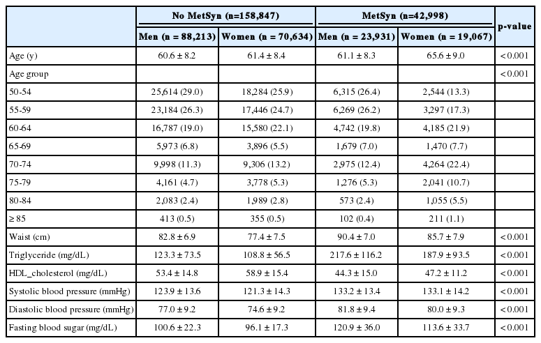
Characteristics of the study population according to metabolic syndrome (MetSyn) status (n=201,845)
직접 표준화 방법을 사용하여 표준화 유병률을 계산하기 위해 먼저 전체 연구대상자를 성별, 연령대별로 분류하였고, 계산에 필요한 각 단계를 Table 2에 정리하였다. 전체 대사증후군의 조유병률은 21.3명(100명당)이었으며, 성별에 따라 차이를 보이지 않았다(Table 2). 전체 대사증후군 표준화 유병률은 21.9명(100명당)이었으며, 성별에 따른 연령 구조를 고려한 후 여자가 11.9명(100명당)으로 남자의 10명(100명당)보다 더 높았다. 남자의 경우 표준화 유병률이 70대까지 증가하다가 이후 감소하였고, 여자의 경우 표준화 유병률이 연령대가 높아질수록 증가하였다(Table 2). Table 2의 결과를 사용하여, 표준화 유병률, 표준오차, 신뢰구간을 다음과 같이 계산하였다.

Standardized rates calculated by the direct standardization method for metabolic syndrome (MetSyn)
먼저 로지스틱 회귀모형을 사용하여 직접 표준화 방법으로 계산한 결과를 손쉽게 도출할 수 있음을 보여주기 위해, 전체 연구대상자를 연령에 따라 50세부터 5세별로 범주화한 연령대(age_gp) 변수(50-54, 55-59, …, 80-84, ≥85)를 정의하였다. 또한 로지스틱 회귀분석을 위해 대사증후군 상태를 나타내는 이분형 종속변수인 ms (= 0: 정상, =1: 대사증후군)를 정의하였으며, 연령대, 성(sex), 그리고 두 변수 간의 상호작용항을 독립변수로 모형에 포함시켰다. 분석에는 R 통계 프로그램을 사용하였으며, 분석 코드는 간단한 주석과 함께 Table 3에 기술하였다.
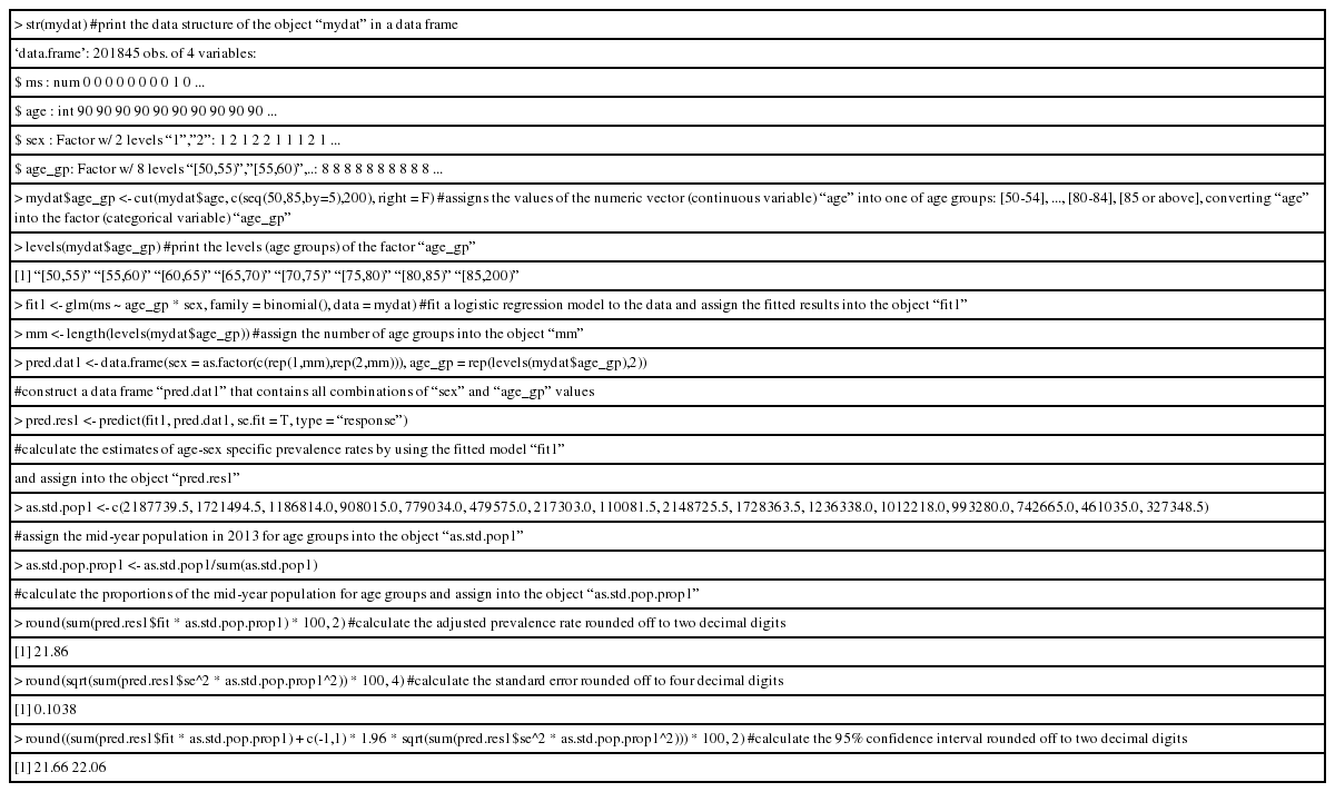
Illustrative R codes for calculating an adjusted prevalence rate by logistic regression analysis: age group as a categorical variable
로지스틱 회귀모형을 사용하여 계산한 표준화 유병률(100명당 21.9명), 표준오차(0.1038), 95% 신뢰구간(21.66, 22.06)은 직접 표준화 방법을 사용하여 계산한 이전 결과와 동일하였다.
다음으로 로지스틱 회귀모형에 범주형 변수인 연령대(age_gp) 대신 연령(age)을 연속형 변수로 포함하여 자료에 적합하였다(Table 4).
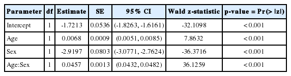
Logistic regression model for metabolic syndrome: age as a continuous variable
적합된 회귀모형을 사용하여 각 성별 연령별 로짓 추정값과 표준화 유병률, 표준오차, 95% 신뢰구간(22.22, 22.31)을 계산하였고, 분석에 사용한 R 코드는 주석과 함께 Table 5에 기술하였다.

Illustrative R codes for calculating an adjusted prevalence rate by logistic regression analysis: age as a continuous variable
연령을 연속형 변수로 모형에 포함하였을 때, 표준화 유병률(100명 당 22.3명)은 크게 달라지지 않았지만, 표준오차(0.024)가 확연히 줄어들었으며, 결과적으로 신뢰구간의 길이도 짧아졌다.
고 찰
로지스틱 회귀모형은 대부분 연관성 분석이나 예측 모형 개발에 사용되고 있으나, 본 연구에서는 로지스틱 회귀모형을 사용하여 유병률을 표준화하는 방법을 소개하였다. 직접 표준화 방법은 범주형 자료에만 사용할 수 있으나, 로지스틱 회귀모형을 통한 표준화는 범주형 변수뿐만이 아닌 연속형 변수를 사용해서도 추정할 수 있다. 연령 변수를 범주화하여 로지스틱 회귀모형에 사용하였을 때는 직접 표준화 방법을 사용했을 때와 동일한 결과를 산출할 수 있고, 연령을 연속형 변수로 모형에 포함하였을 때는 추정량의 표준오차가 줄어들어 신뢰구간의 길이가 짧아지며, 결과적으로 더 신뢰할 수 있는 추정값을 얻을 수 있다. 현재 널리 사용되고 있는 통계 분석 프로그램에는 로지스틱 회귀분석을 수행하는 데 필요한 함수들이 잘 구현되어 있어서, 대용량 자료를 분석할 때, 예를 들어, 다양한 질병의 유병률을 여러 지역별로 산출할 때, 로지스틱 모형을 활용한 표준화 방법이 계산상 효율적일 수 있다. 또한 로지스틱 회귀모형을 통한 표준화 방법은 추정된 모형의 함수관계를 사용하여 자료 수가 부족한 특정 연령대의 유병률도 상대적으로 안정적인 추정을 할 수 있다.
로지스틱 회귀모형에 연령을 연속형 변수로 포함하여 표준화율을 산출하는 방법은 Roalfe et al. [13]에서도 제안되었다. 그렇지만 해당 논문에서는 추정된 로짓에 표준화 인구 분포를 가중치로 부여하여, 결과적으로 표준화 유병률의 추정량은 편향되게 되며, 더 나아가 제시된 신뢰구간이 직접 표준화 방법에 의해 계산된 비편향 추정량을 항상 포함한다는 보장이 없게 된다. 이러한 측면에서 본 연구의 방향과 근본적인 차이가 있다.
로지스틱 회귀모형을 사용한 표준화는 직접 표준화 방법과 비교하여 여러 가지 장점을 갖고 있지만, 직접 표준화에 비해 많이 사용되고 있지 않다. 이 논문을 통해 직접 표준화 방법을 적용하기에 적절하지 않은 상황에서 합리적 대안으로 로지스틱 회귀모형이 널리 사용되기를 기대한다. 또한 본 논문에서 예시로 사용한 자료 분석 결과(Table 2)에서 고연령층에서 더 급격한 유병률의 변화는 관측되지 않았으나, 일반적으로 고연령층에서 유병률의 증가가 더 심할 수 있으므로, 연령층에 따른 유병률의 증가 속도의 변화를 반영할 수 있는 좀 더 유연한 모형에 대한 추후 연구가 필요할 것이다.
Notes
No potential conflict of interest relevant to this article was reported.